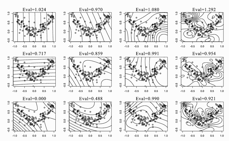
Figure 1: KSIR with Gaussian kernels for the square data. From left to right, the scale of the kernel is set by 0.01, 0.1, 1, and 10. From top to bottom, contour lines of constant value of the first three eigenvectors with the corresponding eigenvalues are shown.

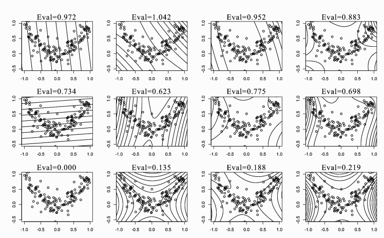
Figure 2: SIR vs. KSIR with polynomial kernels for the square data. From left to right, the polynomial degree of the kernel increases from 1 to 4 (degree = 1 for SIR and degree = 2, 3, 4 for KSIR). From top to bottom, contour lines of constant value of the first three eigenvectors with the corresponding eigenvalues are shown. Note that only two eigenvectors are available in linear SIR.

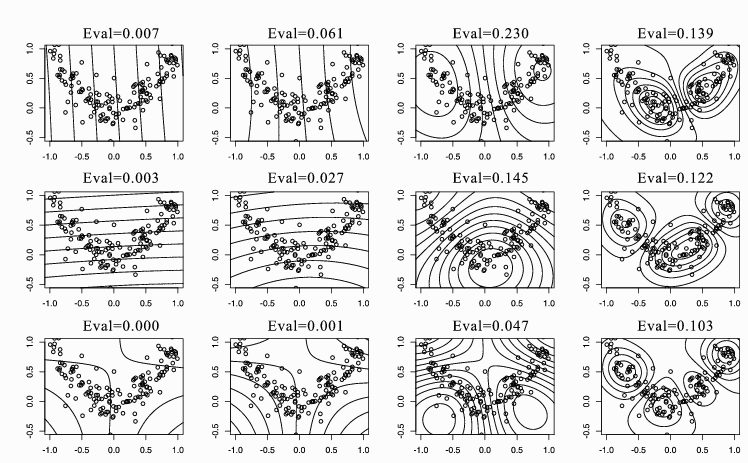
Figure 3: KPCA with Gaussian kernels for the square data. From left to right, the scale of the kernel is set by 0.01, 0.1, 1, and 10. From top to bottom, contour lines of constant value of the first three eigenvectors with the corresponding eigenvalues are shown.

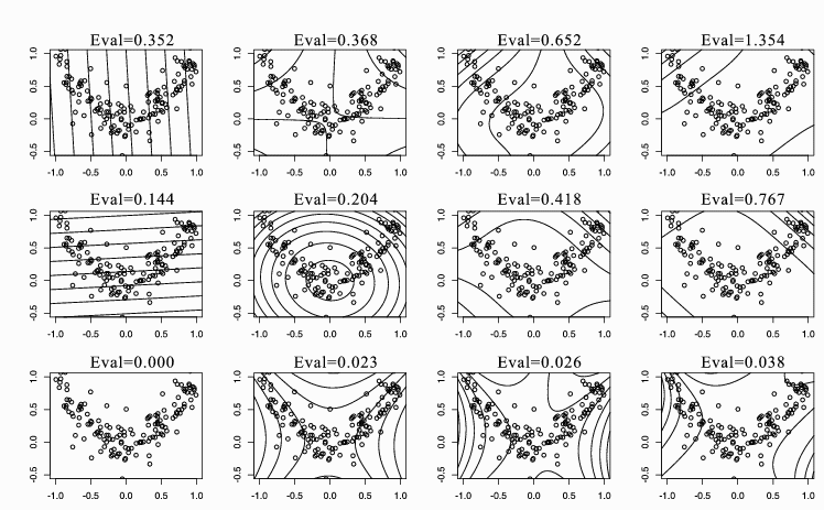
Figure 4: PCA vs. KPCA with polynomial kernels for the square data. From left to right, the polynomial degree of the kernel increases from 1 to 4 (degree = 1 for PCA and degree = 2, 3, 4 for KPCA). From top to bottom, contour lines of constant value of the first three eigenvectors with the corresponding eigenvalues are shown. Note that only two eigenvectors are available in linear PCA.